FARADAY'S LAW OF INDUCTION
It is a basic law of electromagnetism relating to the operating principles of transformers, inductors, and many types of electrical motors and generators. The law states that:
The induced electromotive force or EMF in any closed circuit is equal to the time rate of change of the magnetic flux through the circuit.
Or alternatively:
The EMF generated is proportional to the rate at which flux is linked.
Electromagnetic induction was discovered independently by Michael Faraday and Joseph Henry in 1831, however Faraday was the first to publish the results of his experiments. Expanding on Faraday’s work, James Clerk Maxwell formulated the law quantitatively in the form:
 .
.
where:
 is the magnitude of the electromotive force (EMF) in volts
- ΦB is the magnetic flux through the circuit (in webers).


Example: Spatially varying B-field

Consider the case in Figure 3 of a closed rectangular loop of wire in the xy-plane translated in the x-direction at velocity v. Thus, the center of the loop at xC satisfies v = dxC / dt. The loop has length ℓ in the y-direction and width w in the x-direction. A time-independent but spatially varying magnetic field B(x) points in the z-direction. The magnetic field on the left side is B( xC − w / 2), and on the right side is B( xC + w / 2). The electromotive force is to be found by using either the Lorentz force law or equivalently by using Faraday's induction law above.
Lorentz force law method
A charge q in the wire on the left side of the loop experiences a Lorentz force q v × B k = −q v B(xC − w / 2) j ( j, k unit vectors in the y- and z-directions; see vector cross product), leading to an EMF (work per unit charge) of v ℓ B(xC − w / 2) along the length of the left side of the loop. On the right side of the loop the same argument shows the EMF to be v ℓ B(xC + w / 2). The two EMF's oppose each other, both pushing positive charge toward the bottom of the loop. In the case where the B-field increases with increase in x, the force on the right side is largest, and the current will be clockwise: using the right-hand rule, the B-field generated by the current opposes the impressed field. The EMF driving the current must increase as we move counterclockwise (opposite to the current). Adding the EMF's in a counterclockwise tour of the loop we find ![\mathcal{E} = v\ell [ B(x_C+w/2) - B(x_C-w/2)] \ .](http://upload.wikimedia.org/math/3/b/4/3b462983584a8c265439b7d197e0897f.png)
Faraday's law method
At any position of the loop the magnetic flux through the loop is


The sign choice is decided by whether the normal to the surface points in the same direction as B, or in the opposite direction. If we take the normal to the surface as pointing in the same direction as the B-field of the induced current, this sign is negative. The time derivative of the flux is then (using the chain rule of differentiation or the general form of Leibniz rule for differentiation of an integral):
![\frac {d \Phi_B} {dt} = (-) \frac {d}{dx_C} \left[ \int_0^{\ell}dy \ \int_{x_C-w/2}^{x_C+w/2} dx B(x)\right] \frac {dx_C}{dt} \ ,](http://upload.wikimedia.org/math/e/2/2/e2237b7f8b173cfaa7ca649031d9ee90.png)
![= (-) v\ell [ B(x_C+w/2) - B(x_C-w/2)] \ ,](http://upload.wikimedia.org/math/b/4/f/b4f851ca7be7b782e94cdc5c75b840d5.png)
(where v = dxC / dt is the rate of motion of the loop in the x-direction ) leading to:
![\mathcal{E} = -\frac {d\Phi_B} {dt} = v\ell [ B(x_C+w/2) - B(x_C-w/2)] \ ,](http://upload.wikimedia.org/math/0/c/b/0cbe3a5e31cff775009c21aa909f20e4.png)
as before.
The equivalence of these two approaches is general and, depending on the example, one or the other method may prove more practical.
Example: Moving loop in uniform B-field

Figure 4 shows a spindle formed of two discs with conducting rims and a conducting loop attached vertically between these rims. The entire assembly spins in a magnetic field that points radially outward, but is the same magnitude regardless of its direction. A radially oriented collecting return loop picks up current from the conducting rims. At the location of the collecting return loop, the radial B-field lies in the plane of the collecting loop, so the collecting loop contributes no flux to the circuit. The electromotive force is to be found directly and by using Faraday's law above.
Lorentz force law method
In this case the Lorentz force drives the current in the two vertical arms of the moving loop downward, so current flows from the top disc to the bottom disc. In the conducting rims of the discs, the Lorentz force is perpendicular to the rim, so no EMF is generated in the rims, nor in the horizontal portions of the moving loop. Current is transmitted from the bottom rim to the top rim through the external return loop, which is oriented so the B-field is in its plane. Thus, the Lorentz force in the return loop is perpendicular to the loop, and no EMF is generated in this return loop. Traversing the current path in the direction opposite to the current flow, work is done against the Lorentz force only in the vertical arms of the moving loop, where

Consequently the EMF is

where l is the vertical length of the loop, and the velocity is related to the angular rate of rotation by v = r ω, with r = radius of cylinder. Notice that the same work is done on any path that rotates with the loop and connects the upper and lower rim.
Faraday's law method
An intuitively appealing but mistaken approach to using the flux rule would say the flux through the circuit was just ΦB = B w ℓ, where w = width of the moving loop. This number is time-independent, so the approach predicts incorrectly that no EMF is generated. The flaw in this argument is that it fails to consider the entire current path, which is a closed loop.
To use the flux rule, we have to look at the entire current path, which includes the path through the rims in the top and bottom discs. We can choose an arbitrary closed path through the rims and the rotating loop, and the flux law will find the EMF around the chosen path. Any path that has a segment attached to the rotating loop captures the relative motion of the parts of the circuit.
As an example path, let's traverse the circuit in the direction of rotation in the top disc, and in the direction opposite to the direction of rotation in the bottom disc (shown by arrows in Figure 4). In this case, for the moving loop at an angle θ from the collecting loop, a portion of the cylinder of area A = r ℓ θ is part of the circuit. This area is perpendicular to the B-field, and so contributes to the flux an amount:

where the sign is negative because the right-hand rule suggests the B-field generated by the current loop is opposite in direction to the applied B field. As this is the only time-dependent portion of the flux, the flux law predicts an EMF of


in agreement with the Lorentz force law calculation.
Now let's try a different path. Follow a path traversing the rims via the opposite choice of segments. Then the coupled flux would decrease as θ increased, but the right-hand rule would suggest the current loop added to the applied B-field, so the EMF around this path is the same as for the first path. Any mixture of return paths leads to the same result for EMF, so it is actually immaterial which path is followed.
Direct evaluation of the change in flux

The use of a closed path to find EMF as done above appears to depend upon details of the path geometry. In contrast, the Lorentz-law approach is independent of such restrictions. A discussion follows intended to understand better the equivalence of paths and escape the particulars of path selection when using the flux law.
Figure 5 is an idealization of Figure 4 with the cylinder unwrapped onto a plane. The same path-related analysis works, but a simplification is suggested. The time-independent aspects of the circuit cannot affect the time-rate-of-change of flux. For example, at a constant velocity of sliding the loop, the details of current flow through the loop are not time dependent. Instead of concern over details of the closed loop selected to find the EMF, one can focus on the area of B-field swept out by the moving loop. This suggestion amounts to finding the rate at which flux is cut by the circuit. That notion provides direct evaluation of the rate of change of flux, without concern over the time-independent details of various path choices around the circuit. Just as with the Lorentz law approach, it is clear that any two paths attached to the sliding loop, but differing in how they cross the loop, produce the same rate-of-change of flux.
In Figure 5 the area swept out in unit time is simply dA / dt = v ℓ, regardless of the details of the selected closed path, so Faraday's law of induction provides the EMF as:

This path independence of EMF shows that if the sliding loop is replaced by a solid conducting plate, or even some complex warped surface, the analysis is the same: find the flux in the area swept out by the moving portion of the circuit. In a similar way, if the sliding loop in the drum generator of Figure 4 is replaced by a 360° solid conducting cylinder, the swept area calculation is exactly the same as for the case with only a loop. That is, the EMF predicted by Faraday's law is exactly the same for the case with a cylinder with solid conducting walls or, for that matter, a cylinder with a cheese grater for walls. Notice, though, that the current that flows as a result of this EMF will not be the same because the resistance of the circuit determines the current.
The Maxwell-Faraday equation

A changing magnetic field creates an electric field; this phenomenon is described by the Maxwell-Faraday equation:

where:
 denotes curl
- E is the electric field
- B is the magnetic field
This equation appears in modern sets of Maxwell's equations and is often referred to as Faraday's law. However, because it contains only partial time derivatives, its application is restricted to situations where the test charge is stationary in a time varying magnetic field. It does not account for electromagnetic induction in situations where a charged particle is moving in a magnetic field.
It also can be written in an integral form by the Kelvin-Stokes theorem:


where the movement of the derivative before the integration requires a time-independent surface Σ (considered in this context to be part of the interpretation of the partial derivative), and as indicated in Figure 6:
- Σ is a surface bounded by the closed contour ∂Σ; both Σ and ∂Σ are fixed, independent of time
- E is the electric field,
- dℓ is an infinitesimal vector element of the contour ∂Σ,
- B is the magnetic field.
- dA is an infinitesimal vector element of surface Σ , whose magnitude is the area of an infinitesimal patch of surface, and whose direction is orthogonal to that surface patch.
Both dℓ and dA have a sign ambiguity; to get the correct sign, the right-hand rule is used, as explained in the article Kelvin-Stokes theorem. For a planar surface Σ, a positive path element dℓ of curve ∂Σ is defined by the right-hand rule as one that points with the fingers of the right hand when the thumb points in the direction of the normal n to the surface Σ.
The integral around ∂Σ is called a path integral or line integral. The surface integral at the right-hand side of the Maxwell-Faraday equation is the explicit expression for the magnetic flux ΦB through Σ. Notice that a nonzero path integral for E is different from the behavior of the electric field generated by charges. A charge-generated E-field can be expressed as the gradient of a scalar field that is a solution to Poisson's equation, and has a zero path integral. See gradient theorem.
The integral equation is true for any path ∂Σ through space, and any surface Σ for which that path is a boundary. Note, however, that ∂Σ and Σ are understood not to vary in time in this formula. This integral form cannot treat motional EMF because Σ is time-independent. Notice as well that this equation makes no reference to EMF  , and indeed cannot do so without introduction of the Lorentz force law to enable a calculation of work.

Using the complete Lorentz force to calculate the EMF,

a statement of Faraday's law of induction more general than the integral form of the Maxwell-Faraday equation is (see Lorentz force):


where ∂Σ(t) is the moving closed path bounding the moving surface Σ(t), and v is the velocity of movement. See Figure 2. Notice that the ordinary time derivative is used, not a partial time derivative, implying the time variation of Σ(t) must be included in the differentiation. In the integrand the element of the curve dℓ moves with velocity v.
Figure 7 provides an interpretation of the magnetic force contribution to the EMF on the left side of the above equation. The area swept out by segment dℓ of curve ∂Σ in time dt when moving with velocity v is

so the change in magnetic flux ΔΦB through the portion of the surface enclosed by ∂Σ in time dt is:

and if we add these ΔΦB-contributions around the loop for all segments dℓ, we obtain the magnetic force contribution to Faraday's law. That is, this term is related to motional EMF.
Example: viewpoint of a moving observer
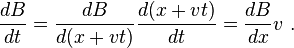
Revisiting the example of Figure 3 in a moving frame of reference brings out the close connection between E- and B-fields, and between motional and induced EMF's. Imagine an observer of the loop moving with the loop. The observer calculates the EMF around the loop using both the Lorentz force law and Faraday's law of induction. Because this observer moves with the loop, the observer sees no movement of the loop, and zero v × B. However, because the B-field varies with position x, the moving observer sees a time-varying magnetic field, namely:
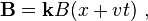
where k is a unit vector pointing in the z-direction.
Lorentz force law version
The Maxwell-Faraday equation says the moving observer sees an electric field Ey in the y-direction given by


Here the chain rule is used:
Solving for Ey, to within a constant that contributes nothing to an integral around the loop,

Using the Lorentz force law, which has only an electric field component, the observer finds the EMF around the loop at a time t to be:
![\mathcal{E} = -\ell [ E_y (x_C+w/2,\ t) - E_y(x_C-w/2,\ t)]](http://upload.wikimedia.org/math/3/b/9/3b950e184ab5d52e2b6aae534a14559a.png)
![= v\ell [ B(x_C+w/2+v t) - B(x_C-w/2+vt)] \ ,](http://upload.wikimedia.org/math/3/c/a/3cacfe084d17fddf872aba14304b720e.png)
which is exactly the same result found by the stationary observer, who sees the centroid xC has advanced to a position xC + v t. However, the moving observer obtained the result under the impression that the Lorentz force had only an electric component, while the stationary observer thought the force had only a magnetic component.
Faraday's law of induction
Using Faraday's law of induction, the observer moving with xC sees a changing magnetic flux, but the loop does not appear to move: the center of the loop xC is fixed because the moving observer is moving with the loop. The flux is then:

where the minus sign comes from the normal to the surface pointing oppositely to the applied B-field. The EMF from Faraday's law of induction is now:


![=v\ell \ [ B(x_C+w/2+vt) - B(x_C-w/2+vt)] \ ,](http://upload.wikimedia.org/math/8/0/3/803906ede26061c543f9a171c6d242e7.png)
the same result. The time derivative passes through the integration because the limits of integration have no time dependence. Again, the chain rule was used to convert the time derivative to an x-derivative.
The stationary observer thought the EMF was a motional EMF, while the moving observer thought it was an induced EMF.
No comments:
Post a Comment